William McDougall

THE tale of my West Gate Tunnel experience is a long one! I’ve broken it up into three parts:

1. The overall story
2. The transport modelling (this post)
3. The cost-benefit analysis

This second post is wordy and somewhat technical. Hopefully, my overview gives you the salient points before diving into more detail. The opinions herein are my own; I encourage you to investigate further for yourselves if you’re interested.

Let me know what you think. I’d be particularly pleased to hear from experienced transport modellers (including Veitch Lister Consulting!) about these issues.

I have some loaded questions for four-step transport modellers reading this post:

• Have you ever checked the convergence of your demand models (in all modelled years and time periods), to see if they meet ATAP requirements (the 0.1% difference in the ‘demand/supply gap’), and to ensure that changes between model loops were less than 10% of the changes due to the project you were assessing?
• If so, what were your results, and what did you do, if anything, to improve them?
• Did you do this through your own initiative, or at the request of a reviewer?
• If you did this and your model did not meet these requirements, did you make that clear to your client, or to those using your results for further analysis?
• Have you ever felt pressured by others for your modelling to produce ‘favourable’ results (perhaps especially when working for toll road bidding consortia)?
• Do you feel resentful or defensive when your hard work is questioned by others?

Overview

Transport modelling for major projects like West Gate Tunnel is a complex process. Good practice has developed over many years, and growth in computing power has made larger models possible.

Here in Victoria, the two most-used strategic, multimodal transport models are:

1. The Victorian Integrated Transport Model (VITM), developed by the State Government; and
2. The ‘Zenith’ model of Victoria, developed by Veitch Lister Consulting (VLC).

VITM is used more for public transport and smaller road projects, while Zenith is used mainly for toll roads, because it’s thought to have better toll diversion modelling. Zenith was used for East West Link, West Gate Tunnel and North East Link.

Zenith uses an unusual and illogical method for future year forecasting, called ‘single loop’ distribution. Essentially it calculates trip distribution (more on that below) by combining today’s travel ‘demand’ with future transport ‘supply’. It also does this only once in the iterative process that the overall modelling method requires, instead of looping through for successively better results.

This means that:

• Zenith significantly overestimates future car-kilometres of travel;
• the model procedure doesn’t comply with established guidance; 
• its mathematical stability and reliability can’t be proven, nor even calculated properly; and
• its outputs therefore shouldn’t be relied upon for cost-benefit analysis.

The single loop method assumes that people make their trip origin-destination decisions as if the transport network was more developed than it is. Conversely, you could say that trip origin-destination decisions are made as if the travel demand on the network had stopped growing sometime in the past.

For most projects, the main forecasting year is 20-25 years into the future, so this effectively means that trip distribution is calculated using the travel demand from 20-25 years earlier. In fast-growing Melbourne, the effect of adding about 2 million more people is therefore ignored during that step of the modelling.

A lot of documentation has been produced in business case and EES paperwork to defend this method, but I still disagree with it. The copious explanations don’t stand up to close scrutiny.

A second problem with Zenith (as used on the East West Link, West Gate Tunnel and North East Link) is that future-year toll prices are lowered, based on an assumption that real wages growth over the last 15 years or so will continue unabated into the future, making prices more affordable. Not only is this a very optimistic projection, it also means that, in the model, toll road users are the only ones who’ll benefit from this, when in reality everyone will. Why not reduce all the other costs (fuel, fares, values of time, etc, etc) in the modelling by the same amount?

In my estimation, these two issues alone mean that forecast traffic on the West Gate Tunnel in 2031 could’ve been overestimated by something like 20-25%, and we can’t assess the reliability of these numbers anyway (due to the convergence issue). The only way of knowing for sure is to re-do the modelling properly.

This error flows through into the economic appraisal, which I’ll cover in part 3.

As it stands, Zenith modelling shouldn’t be relied on for project economics, nor EES impact appraisal. VITM is probably better (it uses the four steps properly, at least), but both models need improvement before being used further.

Most clients, especially Governments, don’t really care about these niceties (in fact most of them won’t even understand them!), especially when the modelling gives them a ‘good result’ for their projects. Unless they do independent, concurrent peer reviews of the work, they have to trust the modellers.

The onus is on transport modellers to do their work properly, and to comply fully with established guidance. We need to lift the game.

What is a ‘transport model’?

In the context of projects like West Gate Tunnel, a transport model is a computerised method of forecasting movements of people and vehicles.

Essentially, a transport model predicts the travel patterns associated with given land uses (demand) and transport provisions (supply) in an area. It enables testing of future changes in both.

The results from such models are used in strategic studies (area-wide), project planning (including business cases) and impact studies (like EESs). They are the main basis for predicting the economic, social and environmental effects of initiatives. Thus, they are central to the selection, justification and environmental appraisal of transport projects.

The Australian Transport and Planning Assessment (ATAP) Guidelines (especially under ‘Tools and Techniques’) contains a detailed description of the minimum requirements for developing and using such models. They result from decades of use and development of transport models worldwide. They have a lot in common with the UK’s Transport Analysis Guidance (TAG).

The four computational steps in a typical transport model are:

1. Trip generation – estimating how many trip-ends will be produced and attracted by all the different land uses in an area;
2. Trip distribution – joining up the trip-ends to create a pattern of trips to and from all the different areas;
3. Mode split – predicting which modes of transport trip-makers will choose for each trip; and
4. Trip assignment – allocating the trips to the area’s transport network so that the demand can be totalled for each ‘link’ in the network.

Each step is calculated using mathematical algorithms which are designed to echo observed travel behaviour. These algorithms use a range of input variables, including travel times/costs, population and job numbers.

Calculation using a four-step model requires iteration, or looping, through the four steps. Each loop uses the results from the previous loop to refine the travel times and costs. A correctly set up model will ‘converge’ mathematically, until the differences between the results from one loop to the next are within specified small tolerances. This is a fundamental requirement of the process. A model which doesn’t converge sufficiently is unreliable and shouldn’t be used for project appraisal.

Before the model can be used to predict future travel, it must be very carefully and thoroughly calibrated to observed conditions, using data collected through physical surveys. These include travel times, traffic counts, public transport patronage figures and household travel surveys. The model’s algorithms have coefficients and equation forms that are carefully adjusted until each of the four steps – and the model as a whole – is as accurate as possible.

It takes a lot of time and money to set up, calibrate and validate a four-step model. In Australia, most jurisdictions have their own, in-house models developed progressively over many years. Some use models developed by private companies, notably the ‘Zenith’ models of Veitch Lister Consulting (VLC).

The Victorian Government has its own in-house model, called the Victorian Integrated Transport Model (VITM), but it also uses VLC’s Zenith model of Victoria. In recent years, the tendency has been to use Zenith for major road projects – especially toll roads – and VITM for public transport projects and smaller road projects. The main reason for this is that VITM doesn’t have a well-developed toll road forecasting capability.

The ‘single loop’

Using Zenith over VITM for toll road modelling means that several unusual quirks of Zenith get incorporated into the process. The biggest of these is the use of an illogical short cut when modelling future years, which I’ll call the ‘single loop’ distribution.

The diagram below shows the difference between the normal four-step process and Zenith’s single loop.

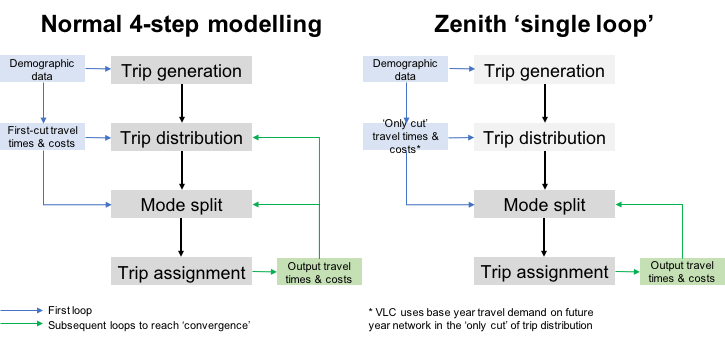
The single loop method combines base year travel times and costs with future year transport network conditions when calculating the trip distribution. It also does this only once. Thus, the future year model only loops through the mode split and assignment steps in subsequent iterations. This conflicts with established practice. It also means that the convergence of the four-step modelling process can’t be calculated, so there is no way of knowing how reliable the future year model runs are.

The single loop method is illogical because it is an artificial situation created by calculating trip distribution on a future-year network by using base year travel times and costs. In a typical modelling exercise, the future years can be 20-30 years ahead of the base year. Why spend all that time and effort to calibrate and validate the model against base year survey data, then use it in a completely different way in future years? 

I was told more recently that this has been a feature of Zenith for a long time. The Zenith model has a very large number of zones, which makes its computation times very long; this would’ve been a much bigger factor with the computers of 25 years ago when Zenith was first set up. Was it originally a time-saving measure?

The convergence issue is important for many reasons:

• ATAP guidance states that the demand model’s convergence should be measured using a specific mathematical test (the ‘demand/supply gap’) which cannot be calculated unless the entire model is looped properly. The results of this test should be less than 0.1% between the final two iterations.
• ATAP also says that the change in network user costs due to a project should be tested using the last two iterations (or by running an additional iteration) to gauge the possible margin of uncertainty in the project benefits, and also to see how much of this difference is due to model ‘noise’. This makes a lot of sense; if the model is too large geographically compared with the project being tested, small but multitudinous differences can crop up in parts of the model which are nothing to do with the project itself. This is rather like background noise in the model which can drown out the effect of the project itself. 
• UK’s TAG goes a little further; it says that the difference in user costs between the last two model iterations must be less than 10% of the change in user costs due to the project being evaluated.

To meet these requirements, these convergence measures should be calculated and reported for each time period the model uses, and for each year the model is run for. They are the acid test of a model’s reliability and validity for project evaluation, yet I know of no-one in Australia who provides such information properly.

In the UK, where concurrent peer reviews are standard practice (and where much of the Australian guidance is copied from), such reporting is mandatory and commonplace. Without it there is no way of knowing whether a model’s results are reliable, nor whether background noise is drowning out the project’s effects. This is fundamental; without it the entire modelling process is open to serious question.

Aside from all this, there’s another major problem with the single loop method. It produces a lot more – and longer – car trips in future years than the correct way of doing it. During the West Gate Tunnel work we were able to compare Zenith with VITM in this regard (VITM loops through the distribution step properly). The models’ results are not too different in the base year (2011), but Zenith produced much more growth than VITM twenty years into the future (2031). When Zenith was run properly (i.e. not single loop) its results were much more consistent with VITM’s.

Note that Zenith covers a larger geographical area than VITM (it includes regional areas around the city), so the last two measures above (km per trip and per capita) are the most relevant for comparing the models.
However, I also question the fact that Zenith has 42% higher car trip lengths than VITM in 2011; this would mean that the average trip length in the regional areas would be nearly 50km, which is definitely excessive, given the vast majority of regional area trips take place within towns and small cities.

The single loop method produced 10% more traffic (car trip-km) than the normal method in 2031. Average car trip lengths increased by 8%, and car trip-km per capita by 10%. This would make the 2031 road network more congested than it ought to have been. Therefore, more traffic would use the West Gate Tunnel.

Notice that, in VITM, car trip-km per capita went down by 9% between 2011 and 2031. In single-loop Zenith, it went up by 3%. 

At the time (i.e. in 2015), VLC argued that car trip-km per capita would increase in the future. This was mainly attributed to Melbourne’s continued urban sprawl. 

A few other reasons were given as well, in this report. During the EES, I wrote some notes on the modelling and related issues for an objector (they were a work-in-progress, and raise many questions which remain unanswered).

This trip-km growth is counter to recent trends. In 2015, BITRE Yearbook data showed that Melbourne’s annual car-km per capita had peaked in 2004 and had decreased steadily since then. The latest BITRE Yearbook, released in December 2019 (just after North East Link’s EES, and before COVID-19), shows that it has continued to decrease. Furthermore, other cities show similar trends.

The graph above shows the BITRE data, and I’ve shown where the trends in the VITM and Zenith modelling would put Melbourne in 2031. Which one do you think is more on-trend?

I wonder how much longer VLC will argue that their single loop modelling is right, while data continues to show that it’s wrong?

As I said already, I was told that the single loop method has been a feature of Zenith for a very long time. Was it originally adopted as a way to shorten computing times, especially in future year runs (of which there can be many, for a given project)?

Deeply buried in the East West Link business case documents (page 1964 of 2022 in the ‘September update’ of 2013), VLC shows that single loop distribution was used on that project, in 2012. No reasons were given for it, nor was it queried by the peer reviewers at the time.

The fact remains that, whether you believe trips will start lengthening again or not (I don’t believe they will), the single loop method doesn’t comply with Australian guidance. It’s a distortion of proper four-step modelling. By definition, a single loop model can’t converge, and its results can’t be relied on for project appraisal. I’m sure that experienced transport modellers would agree with me on that (and I’ve asked a few).

Discounted toll charges

There are other questionable settings in the Zenith model. One particularly problematic one for me is the fact that tollway charges were reduced in future years. This was done in the East West Link, West Gate Tunnel and North East Link models. 

The stated reason for this was that future effective earnings (wages growth ÷ prices growth) were expected to escalate by 1.8%pa over the 20 years from 2011 to 2031, using the same annual growth rate observed from 1995 to 2011. However, the only setting in the model that was changed to reflect this was the toll charges, which were reduced by about 25% for cars and 30% for commercial vehicles in 2031.

This incorrect distortion artificially favours toll road users over everyone else. If earnings are going to increase, everyone will benefit, not just toll road users. All costs in the model, not just the toll charges, should therefore be adjusted to allow for it.

Apart from all that, it’s highly questionable whether the next 20 years will be as prosperous as the last 15, even if we hadn’t had a pandemic. When VLC did the same calculation a few years later for North East Link, the result was to reduce tolls by only 1.55%pa instead of 1.8%pa, because the economy had slowed between 2011 and 2015.

Documents show that this toll charge reduction increased East West Link traffic by 15%. I haven’t found the same information for West Gate Tunnel (the corresponding document hasn’t been released, as far as I can see), but I’d expect a similar result.

Conclusion

The traffic forecasts for West Gate Tunnel were distorted by two main factors:

1. An illogical and non-standard modelling method that produced about 10% more traffic in the model in 2031, compared with the proper way of doing it.
2. An incorrect 25-30% discounting of toll charges in 2031 modelling, making toll roads more attractive than they ought to have been.

I estimate that these issues could have resulted in an 20-25% overestimate of West Gate Tunnel traffic in 2031.

Furthermore, there is no confidence that the modelling is mathematically stable. Because it doesn’t follow normal practice, the key indicator of sufficiently tight model convergence can’t even be calculated.

The over-optimistic traffic forecasts for West Gate Tunnel in turn gave much higher economic benefits for users of the project, thus inflating the benefit-cost ratio.

Some might say that this isn’t important because the future is so unpredictable. I disagree, because these problems are produced through modelling errors. Appraisal tools must be as accurate and error-free as possible so that we can rely on their results, and their stability. Future variations in behaviour, the economy, technology and other things can then be tested by changing the input assumptions.

This brings me to the economic appraisal, in which there are many other distortions apart from those produced by the traffic modelling. I’ll cover these in the next post, in which I’ll also attempt to ‘reverse-engineer’ the West Gate Tunnel’s benefit-cost ratio.

Stay tuned!